Greenhouse Computer Vision and Simulation challenge

As a part of the R&D activity, Quantum Data Science Team took part in Greenhouses online competition. The challenge included two separated stages: Computer vision competition and Greenhouse simulation. The winner was determined by summing up the points for both stages.

Computer vision challenge

The computer vision challenge formulation is quite simple: having RGB and depth images of the lettuce, you need to estimate its fresh weight (grams), height (centimeters), diameter (centimeters), leaf area (square centimeters), and dry weight (grams).

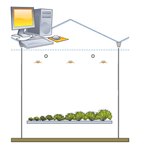
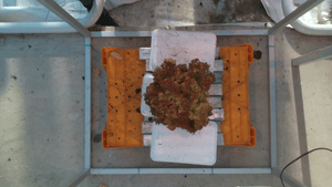
There are 4 lettuce cultivars presented in the dataset: Salanova, Lugano, Satine, and Aphylion. All plants are staying on the same stand and have the same distance between the camera and stand surface (Fig. 1). The target metric for this part of the competition is Normalized Mean Squared Error (NMSE).

Let’s go deeper into the details of our solution. Initially, each image has a resolution of 1920×1080 pixels and contains a lot of useless space. So when we explored the training dataset, we prepared crops of resolution 1000×1000 pixels. According to the training dataset, this resolution guarantees us that any plant will not be cropped. Corresponded fragments were cropped from each depth image. Also, for depth images we determined that lettuce has values between 600 and 1000, so we set to zero all other pixels. Finally, we normalized RGB and depth images, merged them into one 4-channel image, and resized to 512×512 pixels.

As we have 5 target variables with different ranges, we decided to use the natural logarithm of 1 + argument for each of the target variables.

In the modeling phase, we took different classification neural network architectures like ResNet, DensNet and EfficientNet and substituted our head (with 5 outputs) instead of the original one. The EfficientNetB3 model obtained the best performance on the validation set. Our best model showed a 0.065 NMSE score. To extend our training dataset we used image augmentations such as rotations, flips, blurring, crop window shifting and colorspace modifications. One more important thing is that we used a TTA of size 3 on the inference.

As a result of this challenge, we got 0.11 NMSE which is 0.03 worse than leaders have and this score put us into 11th place from 29 teams in this competition.

Simulation challenge

In this stage of the competition, the organizers were required to build a simulation program for the greenhouse simulator. The target metric here is money profit obtained from the greenhouse after simulation, including all costs for the room support and money from the lettuce sale.

The required input is a JSON file with specified controls, including air temperature, humidity, CO2 concentration, heating power, the electricity consumption of lamps, protection screens positions, and so on. One important thing here is that the duration of the simulation was not specified – teams should define it by their algorithms. The output is the score for the current input file and the information about the weather conditions (which were changed after every run).

In general, all teams had 4 simulators named A, B, C and D. Simulator A was used for the model training and was available during all competition time. Simulator B was the validation one and was available once a week for one hour. Simulators C and D – testing instances. C was used on the last day of competition (24 hours) for model fine-tuning. And, finally, leaderboard scores were calculated on the simulator D.

Our approach here was to use the Q-learning algorithm adapted for the current task. We represented all possible controls as states and built a large Q-table based on it. In case we had positive profit, we added it to every corresponding cell in the Q-table; in the opposite case, we subtract 0.1 from every state.

To improve our score and reduce the searching space, we collaborated with a team of greenhouse experts. This team extension allowed us to reduce the possible ranges of the controls to several times.

Finally, we got 23rd place from 32 teams with a score of 5.15 (euro) at this stage. The best team was able to achieve 8.68.

Conclusion

Final result for the competition – 16th place among 35 teams. As we could see from the scores – our computer vision challenge was successful enough. A potential way to increase our score was to use some ensemble techniques or choose another strategy for the validation. But despite this, we had a bad score for the simulation. As we understand now, it would be better to define all available parameters with experts initially before starting to implement models. Another good approach would be to use some optimization algorithms instead of Q-learning.

In any case, this competition was quite useful for us and we got some experience and domain knowledge in a new area – greenhouse analytics and simulation.