Crop type classification with satellite imagery

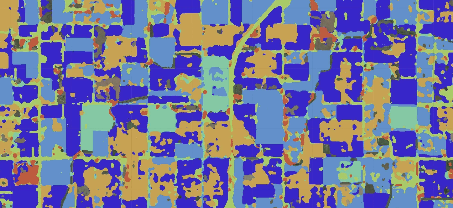
Crop type classification is a common task in agriculture. The main goal of the crop type classification is to create a map/image where each point on it will have a class of what is growing there, as shown in the images below. There are many ways to solve this problem. However, one of the most explored is by using remote sensing data.

There are many articles regarding crop type classification – some of them research the possibility of using multitemporal images – meaning that a time sequence of images is taken instead of an image of one date. Others study the opportunities of using multispectral images, combining images from different satellites, and improving the models themselves.

In our case, we used multitemporal images from Sentinel-1 and Sentinel-2 satellites as model input data. As for the model, we used one of the more common model architectures for segmentation tasks – Unet, along with Conv-LSTM.

Dataset preparation

The dataset for training the model consisted of:

1. Labels – data from CropScape for the 2019 growing season.
2. Model inputs – time sequences of Sentinel-1 and Sentinel-2 satellite images.

We picked the State of Ohio as a study area.

CropScape

1. Top-10 most common classes were used as targets, and all other classes we marked as background. Soybean and corn classes were part of these top-10 classes and were the main crop classes we reviewed.
2. Some of the less frequent classes had to be merged into one to achieve better accuracy, e.g., several types of forest (mixed, deciduous, evergreen) had to be merged into one class. The same procedure was followed for urban areas with different levels of intensity.
3. The final set of classes used during training, validation, and test is the following: corn, soybeans, fallow/idle cropland, urban areas, forest, grassland/pasture, and background.

Sentinel-1

1. We downloaded only GRD products of Sentinel-1 images.
2. Two S1 bands with VV and VH polarization were used.
3. We used the ESA SNAP toolbox to preprocess Sentinel-1 images. The principal purpose of this preprocessing was to run terrain correction of Sentinel-1 images along with noise removal.
4. After SNAP preprocessing, Sentinel-1 images were normalized to bring the values from 0 to 1.

For more details on using Sentinel-1 images, you can read our blog about Sentinel-1 preprocessing.

Sentinel-2

1. Only L2A products of Sentinel-2 images were downloaded.
2. Ten S2 bands were used (blue, green, red, near-infrared (NIR), four red-edge bands, and two short wave infrared (SWIR) bands), and calculated two additional bands commonly used in remote sensing – NDVI and NDMI.
3. All of the twelve bands were normalized to bring the values in the range from 0 to 1.

If you are interested in Sentinel-2 imagery, you can read our blog about our tools for downloading Sentinel-2 imagery.

Data tilling

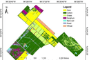
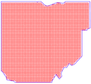
After satellite images were downloaded and preprocessed to be used during training. Big Sentinel images had to be split into smaller images (tiles) (figure. 1). We filtered out Sentinel-2 tiles with a cloud percentage higher than 20%. Sentinel-1 tiles were left as they were. During the training loop, if several Sentinel-2 images overlapped and had a single date of acquisition, only one of the images would be taken to avoid data duplication. The final version of how the State of Ohio was covered is shown in Figure 2.

Modeling

Input features

As described above, we used ten bands from Sentinel-2, two additional index bands, and two from Sentinel-1. We used them during the experiments, and there were no experiments conducted using subsets. Image tiles were 192×192 pixels, and during training, some basic augmentations were applied to them, such as crops, flips, rotations, and resizing. The dataset was split into train, validation, and test sets with a ratio of 70/20/10. A sampling strategy had to be implemented to train on batches of time sequences of images. That would allow us to group sequences of similar lengths into one batch.

Model architecture

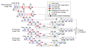
One of the architectures described in this article – 2D U-Net + CLSTM was used. Each satellite has its encoder-decoder-CLSTM model, and later the outputs of each are concatenated and passed into the final linear layer. The architecture of the model from the article is shown in Figure 3.

Hyperparameters

Models were trained using a weighted combination of cross-entropy loss and Dice loss. Adam was used for parameter optimization, with a starting value of learning rate at 0.003 and a reduction of it to 0.0003 after 20 epochs of training. All of the models were trained for 40 epochs total.

Experiments

F1-score metrics were calculated on pixel level for each class separately to evaluate models trained during the conducted experiments. We picked only the metrics for crop classes as they were our main classes, while other classes were supplementary ones to improve model performance on crop classes.

Using different satellite imagery combinations

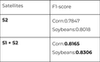
As you can see, the combination of both Sentinel-1 and Sentinel-2 gave slightly better results for our crop classes than using only Sentinel-2.

Using different input resolutions

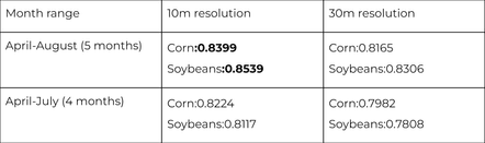
We compared two input resolutions on two different date ranges. In both cases, 10m resolution gave better results than 30m resolution, while the best being a 5-month coverage from the start of April until the end of August.

Using different time frames

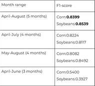
And the final experiment was conducted to confirm that all of the summer growing season gives the best results and to match model performance if the time interval was decreased. It turned out that 4-month range variations reduced the accuracy, but not as poorly as in the case with the 3-month range, meaning that the months when the plants are practically ready to be harvested are much less important than the months when the plants are actively growing.

Conclusion

Consequently, our approaches to dataset preparation and modeling were described. The following comes from the experiment results we got:

1. A combination of optical images (Sentinel-2) and SAR images (Sentinel-1) gives better results than using only optical images.
2. Higher resolution images (10m) give better results than 30m resolution.
3. A date range covering the growing season is much better than shorter dates.