Clearcut segmentation on satellite images using deep learning

Deforestation is a crucial problem nowadays. It can cause climate change, soil erosion, flooding, and increased greenhouse gases in the atmosphere. And such activity as illegal forest logging is one of the main reasons for deforestation. The process of finding these clearcuts consists of downloading images from a satellite, preprocessing the bands, image analysis, and labeling by a person. So there is a lot of manual routine work that can be automated using Deep Learning.

Implementation view

To solve this problem, there has been a solution developed that automatically downloads new images from the satellite storage, preprocesses and prepares data for clearcuts segmentation. Then a deep learning model converts images to binary masks of clearcuts and polygonizes them to vector objects that can be displayed on the map. End users are then able to check each detected clearcut and get statistical information about area changes over time.

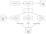
The ClearCut service consists of Image processing and web application back- and frontend.

Image processing

Image downloading

1. Specify image credentials, coordinates, date, clouds coverage, etc;
2. Download channels of the image from the Sentinel-2 server.

Image preparation

1. Filter channels;
2. Create an NDVI band;
3. Scale and concatenate bands into a single TIFF.

Model prediction

1. Load model;
2. Predict segmentation mask;
3. Polygonize the mask;
4. Save polygons and images of the binary mask.

Web application backend

The service’s backend is a simple WSGI application behind uWSGI implemented with Django and Postgres (PostGIS) for storing geospatial data such as polygons. It provides necessary REST endpoints for website frontend which includes:

a. Model call
b. Getting the area histogram
c. Filtering clearcuts by date

Crontab has a scheduled database update (once every 5 days new images are downloaded, processed and the polygons are saved to the database).

Web application frontend

1. Display 3 types of clearcuts:
   a. Data that changed over time
   b. Data that did not change or changed significantly
   c. Data we are not sure about in case of clouds or image issues
2. Filtering by date

Segmentation task

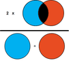
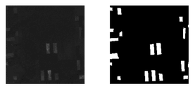
As mentioned before, the process of finding clearcuts is a computer vision task. Each clearcut has its shape and area. So our goal is not only to find the position of a clearcut (object detection) but also to determine which pixels belong to it (semantic segmentation).

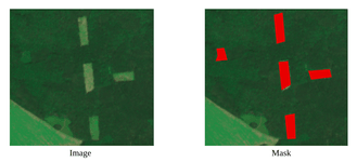
The images above show the example of an input image and desirable output with a separated background and foreground (clearcuts).

Metrics

The first thing we have to establish is our metrics. Metrics give an understandable measure of the solution’s performance. Here are a few metrics that can be used in segmentation task:

Accuracy

The main purpose of segmentation is to separate foreground instances from the background. Accuracy is useless when our classes are extremely imbalanced. In our case clearcuts make up a small portion of the image. So accuracy can be 90% with no clearcuts even detected.

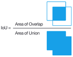
IoU

The Intersection-Over-Union (IoU), also known as the Jaccard Index, is one of the most commonly used metrics in semantic segmentation. In general, the IoU metric tends to penalize single instances of bad classification, which is more informative than accuracy.

Dice score

The Dice score or F score is very similar to IoU but is not as strict. Similarly to how L2 can penalize the largest mistakes more than L1, the IoU metric tends to have a “squaring” effect on the errors relative to the F score. While the F score measures an average performance, the IoU score measures something closer to the worst-case performance. So in our case, it is a more appropriate metric.

Loss function

The second important thing is the loss function. During the training of our machine learning model, we have to change weights in the right direction to get better predictions. In classification commonly used loss function is Cross-Entropy Loss Function. The cross-entropy goes down as the prediction gets more and more accurate. In our case, we predict the class of pixel (background and foreground) and binary cross-entropy shows uncertainty between two classes.

Also to penalize model for miss classifications we add Dice loss with some coefficient to our loss function.

Model architecture

Commonly used neural network architectures for semantic segmentation are U-net, LinkNet, PSPNet and FPN. Here is an easy to use implementation of these models (Keras, PyTorch). You can run the models with different backbones that have pre-trained weights.

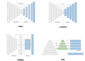
We have tested all of the above with ResNet-50 and ResNet-101 backbones. U-net and FPN with ResNet-50 give the best results on our data. For further improvements, we have tested only on these architectures.

Channels

When working with satellite images, it is a good idea to use additional channels (bands) to increase your model performance. It can be very useful to see these bands on the piece of the map before adding them to your model, so Sentinel-Hub and ArcGis are good options to do some experiments with channels.

We have tested many combinations of the channels (RGB, NDVI, NDVI_COLOR, B2, B3, B4, B8) and the best one is the combination of RGB, NDVI, and B8(infrared). It is the most cost-effective in case of time and memory and gives better results than a simple RGB channel.

Data workflow

The main part of each Machine Learning system is data. We receive raw data and then convert it into a business solution, so it’s extremely important to process our data the right way. The process of working with data for the clearcut segmentation system has multiple steps listed below.

Downloading images from Sentinel-2

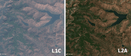
The first thing we have to do is to download raw images from the satellite. In our case, we are working with Sentinel-2 and L2A products. L2A data is atmospherically corrected, with filtered reflectances, so you get a clearer image without additional noise.

For downloading you can use Scihub Copernicus API. In the Net you can find various working solutions that allow you to set parameters for downloading more easily, and here is one of them with two implementations: the first based on Scihub API, and another one based on French mirror.

Data preprocessing

After downloading you have to prepare the data before putting it into your model. In the downloaded archive, you have several different bands, so we have to filter them. Then create an NDVI channel from B4 and B8 bands, scale all bands, convert them into 8-bit images (values of pixel 0–255), and merge them all into a single image. TIFF format is perfectly suitable for storing satellite images. It saves metadata such as geographical coordinates, so you can view images in the QGIS and stores each band as a separate layer.

The original size of the downloaded images with a resolution of 10 meters per pixel is approximately 10K*10K. We can’t work with such big images, so the next step is to cut the whole image into small pieces with sizes 224*224.

Then labeled clearcuts should be converted from GeoJSON polygons to binary masks (0 — background, 1 — foreground or clearcut). You also may not have a fully labeled image, so some of the image pieces won’t have markup, and we have to filter them. We can set a threshold for the percentage of foreground pixels over a total number of pixels on an image to get rid of images with a small amount of useful information. But it is a good idea to leave some non-labeled images to improve model performance on regions without clearcuts such as cities, rivers or crops.

Dataset division

Consider that we have data from different seasons, so we can train different models for each season separately or like in our case-mix data from all seasons together.

After data preparation, we have to divide our data into datasets. The training dataset is the biggest one, usually about 70–80% of all data, the rest goes to validation and testing datasets. Here is a list of techniques that can be used to split your data:

Train/test split

The train/test split is the simplest one. Each image randomly goes to some of the datasets with a fixed probability. We do single division for train-test (70–30%) or multiple division for train-test-validation (70–20–10%).

Stratified split

Stratified split — similar to train/test split, but we also save the balance of classes (areas of polygons). In our case, it didn’t give any significant improvement.

Geographical split

Geographical split — this splitting technique is used when we work with different seasons, which can capture zones that slightly rotated or shifted. We divide dataset by coordinates, so it prevents situations when train data from one season can appear in a test or validation set of another season.

Fold split

Fold split — is just geographical split but by folds. We divide the dataset to a specified number of folds and one additional for the test. Then we use classical cross-validation, which usually gives better results than a simple train/test split.

Augmentations

From one TIFF file (10K*10K) we get 2401 images (224*224) and approximately only 10–15% of them are labeled. It is a really small number of samples for training even if we have images from different dates. So the solution to this problem is to apply some augmentations. Albumentations is a good package with implemented augmentations, which also gives the possibility to easily build pipelines for your preprocessing. In our case, we used RGBShift and CLAHE for RGB band, RandomRotate90 and Flip for all bands. These augmentations increase the number of samples for training to prevent overfitting and not to distort images as much.

Results

Final configuration

Backbone: U-Net with ResNet50.

Dataset: winter (2016.01.03) and summer (2016.06.21, 2016.08.30, 2019.06.26) + 10% of non labeled images to give additional context (get rid of misrecognition in city and other areas).

Channels: RGB, NDVI, B8.

Split function: train/test split (80–20%). We don’t use geo split because we found an area that is not changing over time, so there is no mixing of train and test data in different seasons if we specify the random seed.

Hyperparameters:

• Adam optimizer (lr=1e-3)
• Scheduler (milestones=[10, 20, 40], gamma=0.3)
• Epochs = 100 (we tested 500 and 700 — and model was overfitted)
• Batch size = 8
• Loss function — binary cross-entropy combined with dice score (bce_weitgh=0.2, dice_weight=0.8)

Augmentations:

• RandomRotate90, Flip, RandomSizedCrop for all channels
• RGBShift, CLAHE for RGB channel

Mertics:

• Train
  

  Dice = 0.5757
  Loss = 0.3482

• Validation
  

  Dice = 0.5722
  Loss = 0.3516

On test data without the markup, this configuration gives the best result. We checked performance on different dates, and the version with 100 epochs is not overfitted on winter (on other dates it gives awful results, almost no clearcut is detected).

In addition to the straightforward approach we have tested the next methods:

Multiclass prediction

We can divide clearcuts to such classes as a new clearcut that has more sharp edges and contrast color, overgrown clearcut that was cut many years ago. So our model has to predict masks and classify the type.

Backbone: FPN with Resnet50.

Dataset: Autumn + 2 summers + winter (26.10.16, 30.08.16, 21.06.16, 03.01.16).
Created tiles 320×320 and random cropped 224×224 out of them. Removed “bad” markup from Dataframes.

Channels: RGB.

Hyperparameters:

• Adam optimizer (lr=1e-3)
• Scheduler (milestones=[10, 20, 40], gamma=0.3)
• Epochs = 100 (we tested 500 and 700 — and model was overfitted)
• Batch size = 8
• Loss function — binary cross entropy combined with dice score (bce_weitgh=0.2, dice_weight=0.8)

Augmentations:

• Random rotations
• Random horizontal
• Vertical flip
• RGBShift
• CLAHE

Mertics:

• Train
  

  Dice = 0.4727
  Loss = 0.4476

• Validation
  

  Dice = 0.3873
  Loss = 0.5154

• Test
  

  Dice = 0.5296 (added probabilities from 2 forest cut classes)

Season prediction

Added season prediction as additional output and modified loss function as combination of dice loss and binary cross entropy for season prediction.

Backbone: FPN with Resnet50.

Dataset: Autumn + 2 summers + winter (26.10.16, 30.08.16, 21.06.16, 03.01.16).
Deleted all data where the amount of markup is too small (<0.1% of image size) and data where most of the markup is on the edge of an image.

Channels: RGB.

Hyperparameters:

• Adam optimizer (lr=1e-3)
• Scheduler (milestones=[10, 20, 40], gamma=0.3)
• Epochs = 100 (we tested 500 and 700 — and model was overfitted)
• Batch size = 8
• Loss function — binary cross entropy combined with dice score + binary cross entropy for season prediction. (bce_weight=0.2, dice_weight=0.8, season_weight=0.2)

Augmentations:

• Random rotations
• Random horizontal
• Vertical flip
• RGBShift
• CLAHE

Mertics:

• Train
  

  Dice = 0.634
  Loss = 0.25

• Validation
  

  Dice = 0.607
  Loss = 0.579

• Test
  

  Dice = 0.5124

Autoencoder

We have trained autoencoder on our dataset (also used pre-trained encoder on satellite imagery) and used its weights to initialize a segmentation neural network.

Backbone: FPN with Resnet50.

Dataset: Autumn + 2 summers + winter (26.10.16, 30.08.16, 21.06.16, 03.01.16).
Deleted all data where the amount of markup is too small (<0.1% of image size) and data where most of markup is on the edge of an image.
Created tiles 320×320 and random cropped 224×224 out of them. Removed “bad” markup from Dataframes.

Channels: RGB.

Hyperparameters:

• Adam optimizer (lr=1e-3)
• Scheduler (milestones=[10, 20, 40], gamma=0.3)
• Epochs = 100 (we tested 500 and 700 — and model was overfitted)
• Batch size = 8
• Loss function — binary cross entropy combined with dice score. (bce_weight=0.2, dice_weight=0.8)

Augmentations:

• Random rotations
• Random horizontal
• Vertical flip
• RGBShift
• CLAHE

Mertics:

• Train
  

  Dice = 0.4943 (batch average)
  Loss = 0.4355 (batch average)

• Validation
  

  Dice = 0.5696 (batch average)
  Loss = 0.3750 (batch average)

• Test
  

  Dice = 0.4422 (average)

Folds

We used folds cross-validation for the dataset splitting. It gives some improvement, but we didn’t use it in production, because we haven’t tested it with multichannel images.

Backbone: FPN with Resnet50.

Dataset: Autumn + 2 summers + winter (26.10.16, 30.08.16, 21.06.16, 03.01.16).
Created tiles 320×320 and random cropped 224×224 out of them. Removed “bad” markup from Dataframes.
The data was split using geographical information. The bottom part of the markup/image was taken into the test set. The top part of the image was split into equal pieces between train and validation sets.
Folds distribution number-wise:

1. train: 478, val: 77
2. train: 431, val: 124
3. train: 444, val: 111
4. train: 416, val: 139

Channels: RGB.

Hyperparameters:

• Adam optimizer (lr=1e-3)
• Scheduler (milestones=[10, 20, 40], gamma=0.3)
• Epochs = 100 (we tested 500 and 700 — and model was overfitted)
• Batch size = 8
• Loss function — binary cross entropy combined with dice score. (bce_weight=0.2, dice_weight=0.8)

Augmentations:

• Random rotations
• Random horizontal
• Vertical flip
• RGBShift
• CLAHE

Mertics:

• Train by folds

1. Dice = 0.6543
   Loss = 0.2936
2. Dice = 0.6496
   Loss = 0.3002
3. Dice = 0.6876
   Loss = 0.2650
4. Dice = 0.6667
   Loss = 0.2849

• Validation by folds

1. Dice = 0.6259
   Loss = 0.3251
2. Dice = 0.5970
   Loss = 0.3421
3. Dice = 0.6801
   Loss = 0.2802
4. Dice = 0.6363
   Loss = 0.3080

• Test
  

  Dice = 0.5643

Online service

As a final result, we created a web application that allows monitoring forest conditions. The app reads and processes data from the satellite once every 5 days, performs segmentation, converts results of the polygons and stores the results. End users have the opportunity to view the clear cuts on the map and compare the forest conditions during the time.

The program finds and classifies the clearcuts for a specified period. So users can easily recognize old and new ones.

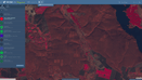
The data displays on the OpenStreetMap (currently just for one region). There we can find the next classes of clearcuts:

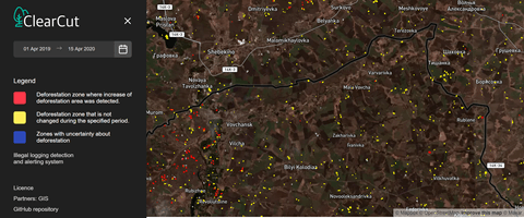
1. Yellow polygon — the deforestation zone that is not changed during the specified period.
2. Red polygon — the zone where there is detected increased area of deforestation.
3. Blue polygon — the zones with uncertainty about clearcuts. Previously there were clearcuts, but now there are not present. Clouds and other variable factors may influence model predictions.

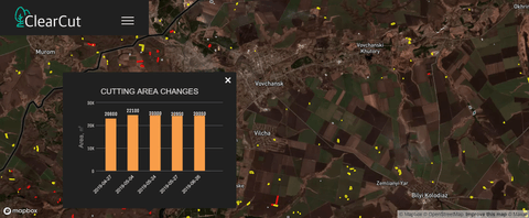
For each clearcut we can plot a graph corresponding to its area changes. When we click the clearcut we get a histogram with deforestation area over time. It helps to determine areas with the most intensive logging.

Conclusion

Deforestation is a big problem, but we have tried to take a step to solve it with modern techniques. Deep Learning is a great tool that can make our planet and lives better. But it is not the final solution, we continue to improve on model performance and accuracy. The project is open-source, so you can contribute as well. We are glad to receive feedback, propositions, and questions from you.

Clearcut Git repository