Using Sigrow Stomata Camera to monitor plant health

Michael Yushchuk
Head of Data Science
Introduction
Greenhouses are an essential part of the modern food supply chain, and their efficiency is a matter of growing concern for growers. Automating indoor climate parameters adjustment is a way to increase the effectiveness of greenhouses and reduce costs. Sounds plain and easy in theory. In practice, however, it gets complicated fast.
Wageningen University & Research (WUR) hosts the Autonomous Greenhouse Challenge, a competition for professional growers, programmers, data scientists, and whoever is passionate about the idea of a challenge. Our data scientists, of course, also participated in it.
Plant stomata: significance of monitoring stomatal conductance for plant growers
Stomata is basically a pore in the plant’s “skin,” which allows the plant to exchange gasses with an atmosphere. Photosynthesis, a process of converting sunlight energy and gasses into sugars, would not be possible without such exchange. Green inhabitants of our planet do not have these pores open all the time. However: whenever conditions are suitable for photosynthesis, the stomata of a plant is open; otherwise, they prefer not to give out water into the atmosphere, and photosynthesis ceases.
Maximizing photosynthesis must be the core objective if growers want plants to grow healthy and produce a good quality product. Monitoring stomatal opening is complicated in its purest form since pores are incredibly tiny. Stomatal conductance, however, is the best indicator of pores opening.
Stomatal conductance is the exchange rate of a particular surface’s carbon dioxide and water vapor. Obviously, the higher the rate, the more actively photosynthesis occurs. The catch is two-fold here: firstly, such a rate is never precisely zero, and the maximum possible value is usually far from theoretical; secondly, it tells nothing about which part of the environment the plant is uncomfortable with, whether it is too cold or too hot, low carbon dioxide level or high humidity. This is where a grower’s knowledge might be of great help.
Hands-on: what insights can we get from the stomata camera?
Image processing is a critical component of many autonomous systems. Whether a self-driving car or a greenhouse, a great deal of information can be gained from images. Organizers of the Autonomous Greenhouse Challenge knew it and took great care of cameras and sensors setup for participating teams.
RGB and Sigrow cameras data overview
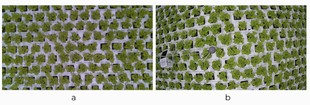
We could operate with two cameras to monitor stomatal conductance: a regular RGB camera and a Sigrow stomata camera. The typical camera had a wide field of view but at the cost of fisheye distortion (figure 1).

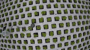
Next to it was situated a Sigrow stomata camera.
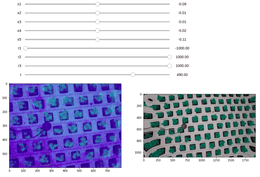
Actually, it senses both stomatal conductance and the temperature of surfaces. At the beginning of the challenge, teams could have only “derived” images, i.e., images where absolute values were normalized to the range of usual pixels from 0 through 255. Later some teams requested raw data with no normalization to be provided. Figure 2 demonstrates both of these sources of data.

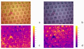
Notice there is a small ball in the pictures. Its purpose is to serve as a reference point, as it has limited transpiration and gas exchange abilities. It shows what values of stomata and temperatures are typical for a leaf with tightly closed stomata, an inactive leaf.
RGB images are far different in nature and in the resolution field of view and have different distortions. To align these two data sources, we needed to develop a slightly more complex flow than regular loading and basic preprocessing.
Image preprocessing and data extraction flow
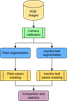
As one might observe, even though there are maps of absolute values, they have no meaning unless there is a mechanism of values attribution. This is where stomatal conductance measures belong to the plant and inactive leaf.
The first step is to locate an inactive leaf. At first, we thought a simple approach would often fail, but it worked repeatedly. What was it? The binary mask of the ball is quickly done with simple graphic tools such as GIMP. We observed that inactive leaf was always around one location. Once we drew a mask and applied it, it became clear it did not move and had the exact location.
The next task is a bit more complex. Which values belong to the plant? Fortunately, we needed a segmentation model for the task of spacing plants out as they grow. But first, we needed to apply camera calibration to make pictures as close to the domain on which the model was trained. Once it is done, the model correctly segmented out lettuce, and this mask was used to locate which values should be considered in comparing the values of inactive leaves and plants themselves. The whole diagram is shown in figure 3.

Camera calibration
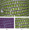
Now, let us dig deeper into the camera calibration and why we needed it in the first place. The segmentation model was trained on regular color images taken by the Intel RealSense D415 camera. Although slightly smaller in resolution, those images had no apparent distortions. An example of it is shown in figure 4.

What camera was that fisheye one? Well, neither we knew nor did the organizers provide us with an answer. It would simplify the calibration procedure if we knew the camera’s intrinsic and extrinsic parameters. What are those parameters anyway? The extrinsic matrix describes the camera’s position and how its lens is situated; it consists of the rotation matrix and translation vector; the intrinsic matrix holds information specific to the camera, such as focal length and optical center. Since we had no such parameters as usually needed for calibration, we tried to approximate them ourselves.
At first, we thought a regular pattern of the holes with plants and known spacing system sizes would help. But once it failed, we developed a tool for manual matrix adjustment (figure 5). Using ten pictures, we selected the most visually suitable parameters and validated ten others.

When the camera parameters are known, we can apply this matrix to undistort images. The results we were able to get are shown in figure 6.

Plants segmentation and localization of inactive leaf
As was mentioned before, a bunch of numbers is still meaningless. To localize the mask, we drew a binary mask that worked perfectly on every sample.
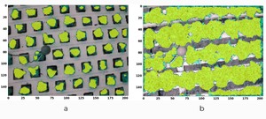
For plant localization and segmentation, a UNet model trained before was used. After the calibration, we could use them on these images. It worked, though not perfectly, leaving out outer regions of leaves but good enough to mask plant values. An overlay of the segmentation mask on the received images is shown in figure 7.

Values extraction and comparison
Finally, we can accurately compare these two when we have both masks for inactive leaves and plants themselves. We took average values across the mask and compared one to another. Typically plants are cooler than inactive leaves, and their stomatal conductance is higher. It is expected, but still, a difference between 0.002 and 0.003 mmols/(m2 · s2) is strikingly different from 0.001 and 0.12. We decided to get a relative difference in percentages to get a broader picture. As a result, we could get a better insight into the tendencies and range of values.

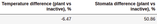
Result: history of stomata and thermal profiles
There inevitably will be periods characterized by different conditions: temperature inside the greenhouse, radiation level plans are exposed to, humidity levels, and many more. This is undoubtedly reflected in the stomata conductance values. Now, I will not bore a reader any longer and will show the progress of our lettuce over time, as well as stomatal and thermal values and deliverables.

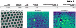

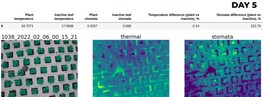

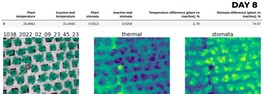

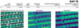

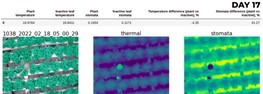
As we can see, the tendency of stomatal conductance difference gets smaller as a plant grows. Notice that not only stomatal conductance is different for plants but an inactive leaf as well. Why is it? Because this rate differs depending on numerous factors such as temperature, pressure, humidity, air composition, and much more. But this is a topic that deserves an article of its own.
Conclusions
Stomata opening is a crucial part of the plant development process. There are well-measured metrics that are an excellent proxy of the phenomenon. One such measure is stomatal conductivity which can be measured with the use of a stomata camera.
Such a camera alone cannot give a grower helpful information as stomatal conductivity depends on numerous factors. The better approach is to localize the inactive leaf and plant segmentation with the consequent masking of values.
Different ranges of stomatal conductivity values characterize different stages of growth. This should be taken into account for adequate assessment of obtained measurements.