New Ways to Recognize Agricultural Patterns from Aerial Images

Anastasiia Dolgaryeva
Delivery Manager
In April 2020, our team participated in the first Agriculture-Vision Challenge. The Challenge, organized by IEEE/CVF CVPR, was aimed to encourage research in developing novel and effective algorithms for agricultural pattern recognition from aerial images.
Having extensive expertise and considerable experience in collecting and analyzing data from satellites, drones, and sensors for our customers within the agritech industry made us accept the challenge and try our hand at innovative pattern recognition.
Because our team of 3 people started the competition a bit later than others, we were left with only 4 weeks to provide a solution. In the end, we managed to reach the middle of the leaderboard and ended up 18th out of 36 teams with an mIoU 0.521 (ranges from 0-1). Quite close to the 1st place solution at 0.639. Our final submission consisted of an ensemble of models, and the best single model score achieved was 0.5. In this article, we’ll focus on this particular model. Other competitors’ solutions can be found in the challenge summary paper.
Competition description
The competition put forward a semantic segmentation task for the following 7 classes:
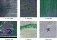
- Cloud shadow;
- A double plant (extra plants, e.g. a grid instead of lines);
- Planter skip (skipped plants, e.g. a skipped row);
- Standing water;
- Waterway (a strip of grass in between fields used for water drainage);
- Weed cluster;
- Background.
A slightly modified mean Intersection over Union metric was used to compare solutions since some classes could overlap. In these cases, a correct prediction would count as a prediction of any of the ground truth classes for the given pixel.

The equation for the metric; Pc and Tc are predicted and ground truth masks correspondingly.

Data exploration
In the dataset, 12,901 training images were provided, 4,431 validation images, and 3,729 test images. A whitepaper describing the process of dataset collection can be found on arxiv. The images have 4 channels: 3 visible spectrum channels — RGB and one near-infrared channel — NIR.
Class imbalance


The classes were highly unbalanced, especially in the case of planter_skip. For this class, we had fewer than 400 labels. At the same time, weed_cluster—a class with the highest number of labels—had over 8,000 labels.
Labeling quirks
Labels provided in the dataset were created by what seems like several different people with different understandings of the classes. This was particularly noticeable in the weed_cluster and planter_skip classes. Furthermore, labels were masked by field boundaries and valid data masks. The full original labels were not provided. You can read more about this issue in this thread. Some masks also exhibited artifacts. We had to remove them from the training process, which has improved the overall training.
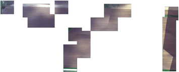
-
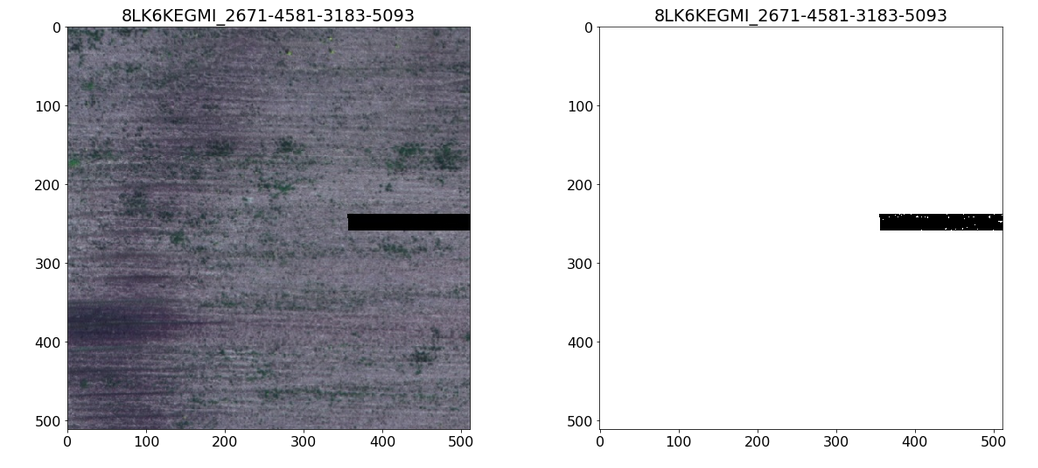
Artifacts in the masks. Note noise in the mask and its absence in the image.
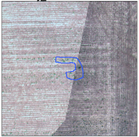

Inaccuracies in labels.
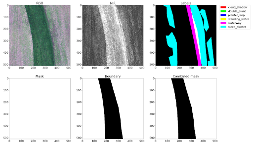
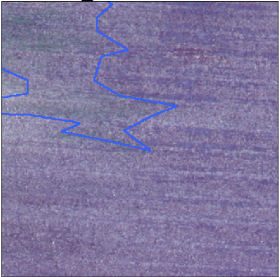
Example of boundary “cutting” a class.
Sometimes, labeled areas are way bigger than the class (weed cluster in this case).
Adversarial validation

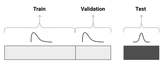
Armed with the knowledge from data exploration and a small baseline model (which had a pretty bad score), we decided to perform adversarial validation on the provided dataset. The aim of adversarial validation was to figure out whether the training and the test datasets came from different distributions. In this particular case, we wanted to know if the labeled part of the dataset came from the same distribution as the unlabeled “test” part.
If the distributions were different, we would choose images most similar to the test set to serve as a local validation set. Doing this would ensure that our local score measurements correlated with the leaderboard. Otherwise, we could use the provided split as is.
To figure this out, we merged the train, and the validation sets into a single “train” set. Then we created a simple binary classifier to distinguish the “train” and the “test” sets. If the classifier could distinguish the two, the distributions were different. If not, they were the same.
After training the classifier and measuring ROC-AUC, we got a value quite close to 0.5. This indicated that the distributions were very similar and the splits could be used as-is.
Solution
The best model can be summarised as follows: csse resnet50 fpn, with a classification head and correlation operations in the bottleneck and all skip connections, with rgb-ndvi input, mosaic oversampling of planter_skip class and tuned thresholds. Let’s go over each part one by one.

Model architecture
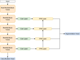
We used one of the classic segmentation architectures — a Feature Pyramid Network (FPN). We chose a fairly standard resnet50 backbone and added Concurrent Spatial and Channel Squeeze & Excitation blocks right before each downsampling operation and at each step in the feature pyramid. This combination worked really well for us in our previous similar projects, so it was a solid bet for this competition.
We added a classification head to the network’s bottleneck. An approach we picked up from kaggle competition solutions. This adds an additional loss to the bottleneck and is supposed to improve gradient flow through the network. In addition, the classification results could be used to filter out noise from the segmentation outputs (although this filtering didn’t help much in our case).

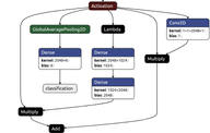
Inspired by the FlowNet paper, we added a “correlation” (“Corr Layer” in the illustration above) operation into the bottleneck and all of the skip connections. Some classes were quite context-dependent, so considering a certain relationship between a pixel in the image (or a feature map in our case) and all the others should improve model performance. Fortunately, the tensorflow_addons repository has the layer implemented as CorrelationCost, so it is just a matter of putting it in the right place and choosing a good set of parameters. We have never seen this approach applied to a segmentation task.
Using the NIR channel
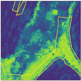
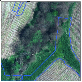
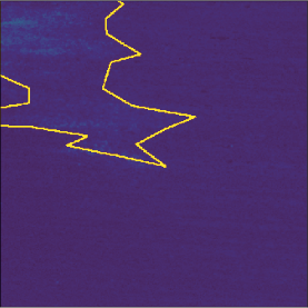
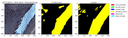
To make use of the extra NIR channel, we calculated NDVI and added it as an additional channel to the RGB input. NDVI is a common index used for agricultural image processing. NDVI ranges from -1 to 1, where values closer to 1 represent more “plant-like” pixels.


RGB on the left. NDVI on the right. Note how much easier it is to see plant matter on the NDVI image.
Oversampling
The dataset provided was cut with overlap from a set of large rasters. Luckily, the dataset split was fair, and different fields were chosen for each subset. Here we attempted to reconstruct the rasters and do random crops around the rare classes, in particular, the planter_skip class. Cropping from reconstructed rasters allowed us to take crops “between” the training examples, which created a more diverse dataset.

Thresholding
Since the classes were not mutually exclusive, we had to choose a threshold for each one separately. For each class, a set of thresholds 0.1-0.9 with a step of 0.1 was checked, and the highest-scoring one was chosen.
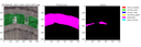
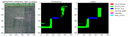
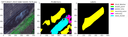
Prediction examples


Conclusion
Despite labeling quirks and time constraints, our model is able to provide predictions useful for downstream tasks. We believe that further improvement can be achieved given higher-quality labeled data and larger-scale computations. Incorporating ideas from other participants might also improve results. For example, using expert networks and task-specific loss functions helped other participants in the competition.
Contact us if you have questions or ideas, and follow our blog updates.
Read more: Precision Agriculture Technologies: Variable Rate Application