DIY Audio Data Processing: Wake Word Detection and Sound Classification

Aleksandr Dolgaryev
CTO
We’re all used to smart home assistants now: they execute voice commands, alert us about suspicious activities, and tell jokes. Basically, many of us can buy it now – the price range is vast. But wouldn’t it be exciting to build one yourself? Well, not the entire assistant, but at least a custom audio processing system no smart assistant can function without.
In this article, we’ll give you a jump-start on how to create your own audio processing system. It includes steps to develop a system that uses an audio stream from a connected microphone and sends out alerts when a keyword was spotted or a target sound (e.g., a baby crying) was detected. Shall we?
Audio data
First, let’s define audio data.
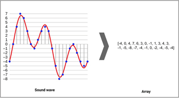
According to Wikipedia, sound is a vibration that spreads as an acoustic wave through a transmission medium (gas, liquid, or solid). But for sounds to become audio data, they need to be digitized by sampling them at discrete intervals, aka the sampling rate. The rate for CD-quality audio is typically 44.1kHz, which means that samples are taken 44,100 times/second.
A sample equals the amplitude of the wave at a certain time frame. The bit depth determines the dynamic range of the signal, meaning that it shows how detailed the sample is. Usually, it’s 16bit – 65,536 amplitude values.

Audio dataset
Existing audio datasets
When you think about starting an audio processing project, the first thing you think of is where to get the data, especially if you’ve only worked with tabular data and/or images before. No need to worry – there are plenty of audio datasets that can be used for research purposes. Here are some of them:
ESC-50
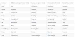
The Environmental Sounds Classification dataset is a goldmine. Also known as ESC-50, this collection of 2,000 labeled recordings of environmental sounds is great for benchmarking different methods of environmental sound classification.
The dataset consists of five-second-long recordings organized into 50 semantical classes (with 40 examples per class) loosely arranged into five major categories:
- Animals
- Natural soundscapes and water sounds
- Human, non-speech sounds
- Interior/domestic sounds
- Exterior/urban noises


Google Speech Command
TensorFlow and AIY teamed up to give the world the Speech Commands Dataset – a free dataset beginners can use to train. Where else would you easily get 65,000 one-second long utterances of 30 short words by thousands of people? Thanks to the dataset, you can build basic voice interfaces that include words like “Yes,” “No,” digits, and directions.
There’s even a tutorial provided by TensorFlow on how to build a basic speech recognition network that recognizes ten different words.
Freesound
Creative Commons is a license that allows sharing, using, and altering a work without violating the copyright, and Freesound is a collaborative database that allows just that. You’re free to browse, download, and share all sounds on Freesound, from special effects to human voice samples.
Data collection
If your task is more specific and requires additional data collection, you can get help on freelancing websites. Quantum needed to collect platform-related voice commands, and we used Amazon Mechanical Turk. Although there was no pre-made audio collection template out-of-the-box, there are plenty of instructions on the web on how to create one.
Audio processing
When you have all data ready, it’s finally time to start working with it.
Dataset evaluation
The first thing you should do in any type of project is to see what data you have and understand it. In the case of audio, you need to listen to what you have in order to evaluate its quality and variety. If the data was collected on a freelance platform, we recommend evaluating every record as the quality of the submissions might not be the best. In case you’re using an already available dataset, listening to a couple of samples is also a good idea. Most issues are usually associated with “noisy” data.
Getting started
Below are simple examples of where to start with both packages.
This is how to load an audio file using Librosa. X is a NumPy array representation of the input audio file. It is an (N, SR) shaped array, where N is the number of channels (1 for mono, 2 for stereo), and SR is Sample Rate that defaults to 22100:
import librosa
audio_path = 'audio-path'
x , sr = librosa.load(audio_path)
And this is how you can use Pydub to load and listen to a file in Jyputer Notebook:
from pydub import AudioSegment

audio = AudioSegment.from_file("file.wav", "wav")
You can use this “data visualization” when filtering files instead of using standard audio players.
Dataset preprocessing
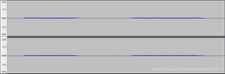
The first thing you should do is clear all the target samples of silence. It’s easy to do using Librosa, but you need to play with the top_db threshold – the default one didn’t work in our case.
Removing silence
y, sr = librosa.load(file)
yt, index = librosa.effects.trim(y, top_db=20)
y_harm, y_perc = librosa.effects.hpss(yt)
librosa.display.waveplot(y_harm, sr=sr, alpha=0.25)
librosa.display.waveplot(y_perc, sr=sr, color='r', alpha=0.5)
plt.title('Harmonic + Percussive')
plt.tight_layout()
plt.show()
Raw audio:


Trimmed audio:

Audio normalization
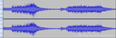
Since all data consists of the target sounds only, we can use Pydub to normalize it, just like in classic Machine learning. Here is an example:
from pydub import AudioSegment, effects

rawsound = AudioSegment.from_file("input.wav", "wav")
normalizedsound = effects.normalize(rawsound)
normalizedsound.export("output.wav", format="wav")
Raw audio:

Normalized audio:

Feature extraction
When the data is fully filtered and clean, it’s time to create features from the raw audio files.
There are plenty of features available in the Librosa library for that. Here are the ones we chose for our task, but you can choose differently:
y, sr = librosa.load(audio_file_path)
chroma_stft = librosa.feature.chroma_stft(y=y, sr=sr)
rmse = librosa.feature.rms(y=y)
spec_cent = librosa.feature.spectral_centroid(y=y, sr=sr)
spec_bw = librosa.feature.spectral_bandwidth(y=y, sr=sr)
rolloff = librosa.feature.spectral_rolloff(y=y, sr=sr)
zcr = librosa.feature.zero_crossing_rate(y)
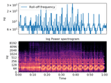
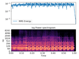
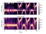
mfcc = librosa.feature.mfcc(y=y, sr=sr)And here is a visual representation of some of the features created:

Modeling
If you need the system to run on an embedded device, such as Raspberry Pi, especially along with other modules like Object detection on a video stream, you need to consider the size of the models you use. It was the case for us, so the tested models ranged from Scikit-learn LogisticRegression to simple neural networks.
Sound classification
The sound classification task we have as an example is implementing an automated baby monitor-like system that goes off when a baby’s cry is spotted. The data we used for this task is the DonateACry corpus.
Classifying the sound of a crying baby is quite easy since it’s distinctive and hard to confuse with anything else. Plus, we wanted to keep this module small for better performance on an embedded device. That is why we applied Scikit-learn Logistic Regression, Gaussian Naive Bayes and Random Forest Classifier.
The features taken from audio samples are:
- ‘chroma stft’
- ‘mfcc’
- ‘rolloff’
- ‘spectral bandwidth’
- ‘spectral centroid’
- ‘zero-crossing rate’
Here are the results for the trained models for sound classification:
| Precision | Recall | F1-score | Time reference* | Feature creation time** | |
| Logistic Regression (all features) | 0.99 | 0.99 | 0.99 | 0.0004s | 0.050s |
| Gaussian Naive Bayes (all features) | 0.98 | 0.99 | 0.98 | 0.0005s | 0.050s |
| Random Forest (all features) | 0.99 | 0.99 | 0.99 | 0.5s | 0.050s |
* Time that takes to predict 1,000 audio files (for a performance reference)
** Time that takes to preprocess an audio file to be a valid model input
Wake word detection
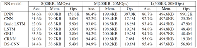
There were ~1,500 audio files collected on Amazon MTurk for custom wake word detection. Seven different model architectures were used, and three different model sizes. The models were trained using the Keyword Spotting repository, which is targeted at embedded devices with Arm processors.
This is the results of training the model on the Google Speech Command dataset alone:

And here are the test metrics for models trained on collected custom data (medium models only):
| Precision | Recall | F1-score | |
| Basic LSTM | 0.92 | 0.96 | 0.94 |
| CNN | 0.92 | 0.97 | 0.94 |
| CRNN | 0.93 | 0.97 | 0.95 |
| DNN | 0.85 | 0.97 | 0.91 |
| DSCNN | 0.94 | 0.98 | 0.96 |
| GRU | 0.90 | 0.95 | 0.93 |
| LSTM | 0.92 | 0.97 | 0.94 |
Postprocessing
You can apply different processing method tricks to decrease the False Positives rate. First, take a sliding window of the audio stream and check consecutive audio frames to compare the results – it removes most of the FP if the model is well-trained. Then, take an even smaller sliding window and set a threshold of the number of consecutive frames to trigger an alert in the system. It’s also a good idea to set the audio volume threshold to skip through the silent/quiet parts of the stream.
Stream processing
Now that we had all of our models trained and tuned, we needed to create the audio processing pipeline itself. There’s a convenient setup in PyAudio to process an audio stream. The created stream has a callback option where you can infer the models using input data. You can also tune the parameters to have the sliding window mentioned in postprocessing.
# instantiate PyAudio (1)
p = pyaudio.PyAudio()

# define callback (2)
def callback(in_data, frame_count, time_info, status):
data = wf.readframes(frame_count)
return (data, pyaudio.paContinue)

# open stream using callback (3)
stream = p.open(format=p.get_format_from_width(wf.getsampwidth()),
channels=wf.getnchannels(),
rate=wf.getframerate(),
output=True,
stream_callback=callback)

# start the stream (4)
stream.start_stream()

# wait for stream to finish (5)
while stream.is_active():
time.sleep(0.1)
Final words
While all of the methods are legitimate and aimed at a successful result, during real-life testing using an audio stream from the target device, you might encounter certain issues.
For example, the dataset might not be balanced to take into account the realistic audio feed: silence and/or background noises. It can be either fixed by creating rules in the audio processing pipeline or by incorporating the negative samples of the dataset. The target device (e.g., microphone) can also differ from the one used to record the data, this is why there is a need to conduct additional tests on the target platform itself.
And this is how you work with audio data in data science projects. We hope that our quick-start guide will help you with your audio-related projects. You can also try it out as a less ordinary research project. And stay tuned for more experiments from the Quantum team.
Read more: Accents classification with DNN