Preparing Aerial Imagery for Crop Classification

Anastasiia Dolgaryeva
Delivery Manager
The first time I had the idea of creating this article was when I started analyzing satellite and aerial images with the help of Computer Vision. At that time, I did not find any complete guide on the topic or even data description and processing methods for further analysis. To this day, there is a long and tedious search awaiting Data Scientists who want to dive deeper into this sort of analysis. They need to find out what GeoTIFF and GeoJSON, how to generate a binary segmentation mask or convert raster and vector to the same WGS. In this article, I will try to shed light on these issues and many more.
All the code is available at Google Colab and GitHub. Feel free to try it out yourself!
Data
All of my explanations are centered around the current Zindi: Farm Pin Crop Detection Challenge. Let’s get started.
First of all, we need to download the data. There are two archives that we will use: train.zip containing GeoJSON and 201–01–01.zip containing GeoTIFF files. All of it is open-source data from the Sentinel-2 satellite. Inside you will find .jp2 files.
GeoTIFF
Let’s find out what GeoTIFF is. Wikipedia says:
GeoTIFF is a public domain metadata standard that allows georeferencing information to be embedded within a TIFF file. The potential additional information includes map projection, coordinate systems, ellipsoids, datums, and everything else necessary to establish the exact spatial reference for the file. The GeoTIFF format is fully compliant with TIFF 6.0, so software incapable of reading and interpreting the specialized metadata will still be able to open a GeoTIFF format file.
You can explore geocoding and other technical details here. But, to put it simply, GeoTIFF is a Raster image with geographical reference. This means each pixel in the image is tied to a real point on the world map.
Working with GeoTIFF
Software
Rasters usually have large sizes, to open them, you need to use specialized software like ArcGis, or its open-source brother QGIS. You can find the QGIS installation guide following the link.
Libraries
There are two main libraries to work with georeferenced images in the Python ecosystem. They are GDAL and Rasterio. GDAL is an older C++ library, which is faster and has more capabilities. But Rasterio is much easier to use for Python developers, that’s why we will use it in Rasterio.
Reading raster files
Let’s open the .jp2 file:
After executing this block, you must see the raster image shape and meta:
Metadata contains the number of bands in the raster, coordinate system, dtype, driver nodata, and transform — all of these fields are straightforward except for transform. “Transform” is an Affine object that creates image geographical referencing. Again, simply put, it is an affine transformation of image coordinates to a world geographical system.
Reshaping rasters
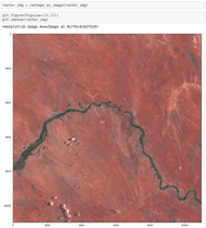
Rasterio reads raster in a differing from usual (OpenCV, Skimage) channel order (num_channels, width, height) instead of (width, height, num_channels). But luckily, Rasterio has a function that transforms it into a familiar and nice shape. Let’s use it and check the results:
Opening the labels
And now when we got a basic understanding of what a Raster is, let’s check what the labeling looks like. Usually, the labeling is stored in .geojson or .shp formats. GeoPandas will help us read it.
The main difference between Pandas vs GeoPandas is that GeoDataframe has to have a ‘geometry’ column. This column contains a Shapely geometry object like Point, LineString, Polygon, or Multipolygon. Shapely is a library to work with vector data — applying operations like cut, intersect, unite, etc, and doing it very efficiently, because of the vector format of data.
Data masking using Rasterio
As you can see, the Polygon (2467881.175041331 …) coordinates are in the World Geographical System. Keep in mind that we need to solve a classification task. Let’s prepare the data, cutting each field from a map. For this purpose, Rasterio has a function called the mask.
Rasterio failed to mask the data. The problem is that .shp CRS doesn’t match the CRS of the raster. We need to convert them manually. First, let’s determine the current projection of Polygons. Take some points from the polygon as an example:
- Go to http://projfinder.com/
- We know the data came from South Africa let’s zoom into it.
- Use it with any coordinates (for example, X: 2467881.175041331 Y: -3352032.059296422) from the GeoDataframe and check the output. We are looking for a place in South Africa, that has a river — we can see it in our image. Looking through the results, we will see one that fits:
EPSG:3395 Name: WGS 84 / World Mercator.
Now let’s check the masking again:
Now you see only 150 masks weren’t masked well. Those fields came from neighboring tiles, to make them also work, you need to download the file: 2017–01–01-JFP.zip. Merge it with the current raster and repeat the procedure.
Now you have a folder with a dataset similar to MNIST, which consists of raw images for train and labels in traindf. Looks like we are done. It is time to take your favorite framework and train some neural networks.
Data preparation
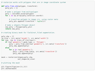
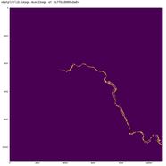
If you want to make semantic segmentation not to just classify the fields but also to find their boundaries, you can do a field/not field binary segmentation or a more complex multiclass segmentation for each class binary mask. Let’s prepare data for semantic segmentation! One solution for this is to convert vector polygons to raster and then cut it into tiles. We will use the function rasterio.rasterize.
Let’s save this binary mask. Here you must remember that the new raster has 1 channel instead of 3 and update .meta, respectively.
I will leave preparing the data for multiclass segmentation to the Reader as a small home task =)
Now you can cut TCI raster and mask to tiles and use them to train your segmentation model.
Conclusion
In this article, I tried to provide the Reader with some basics on preparing aerial/satellite images for some Computer Vision processing. Gave some knowledge on how to work with most-used data types as .shp, .geojson, .tiff, .jp2 using satellite data competition as an example. Also, I described some major pitfalls, that newcomers can meet. I hope it will help you start off faster with the new data type.
Contact us if you have questions or ideas, and follow our blog updates.
AI & Machine Learning
Automate repetitive visual monitoring to boost operational efficiency, reduce costly human error, and accelerate core business workflows.
Check the service

